揭阳网站制作多少钱小游戏代理平台
目录:导读
- 前言
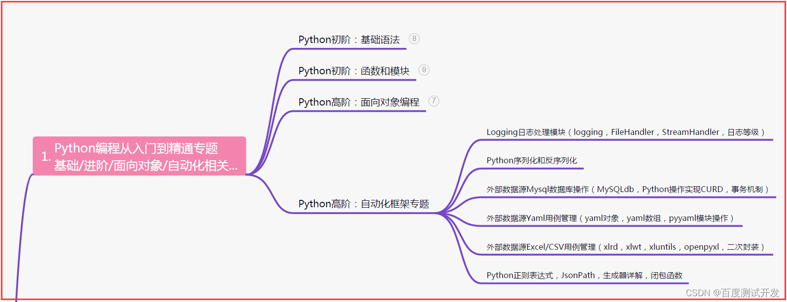
- 一、Python编程入门到精通
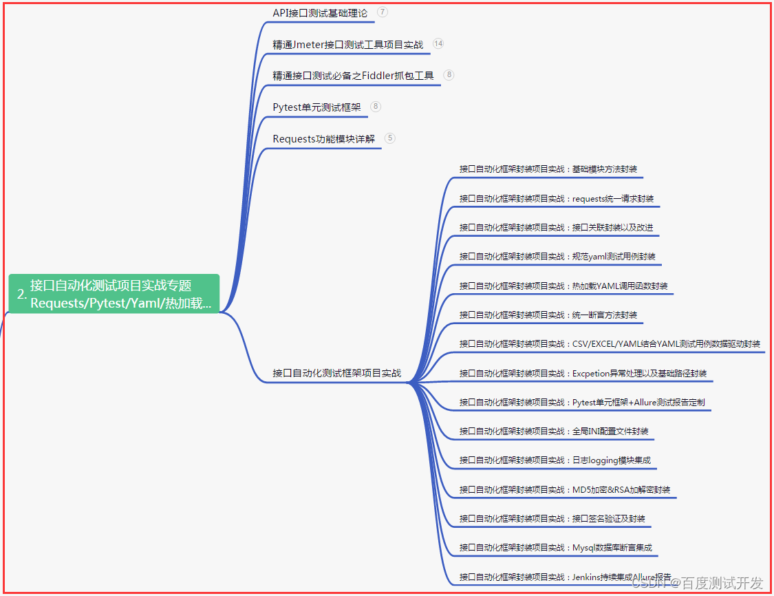
- 二、接口自动化项目实战
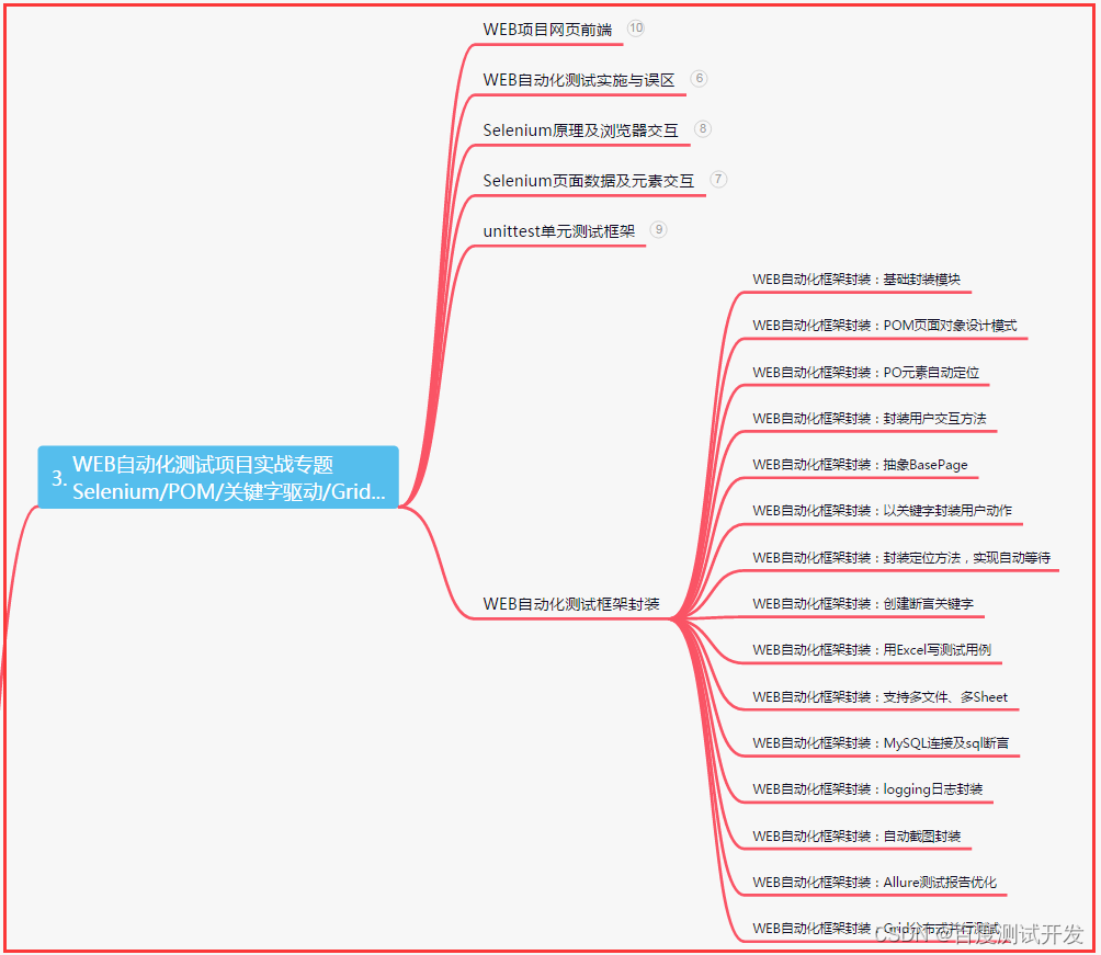
- 三、Web自动化项目实战
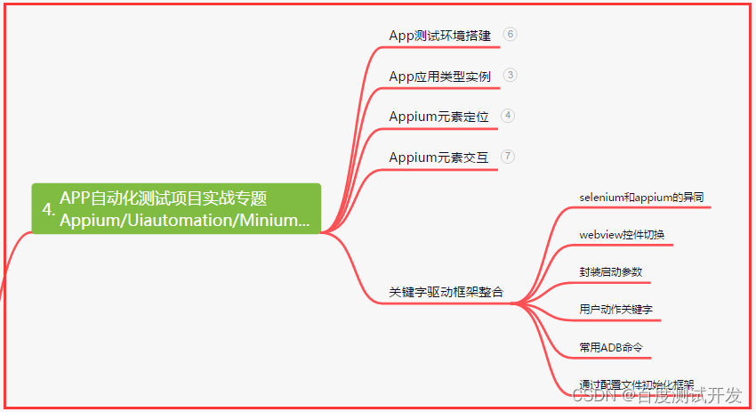
- 四、App自动化项目实战
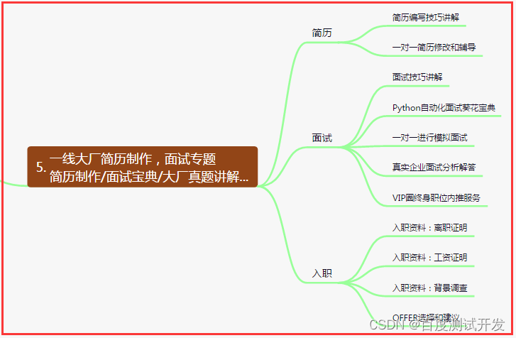
- 五、一线大厂简历
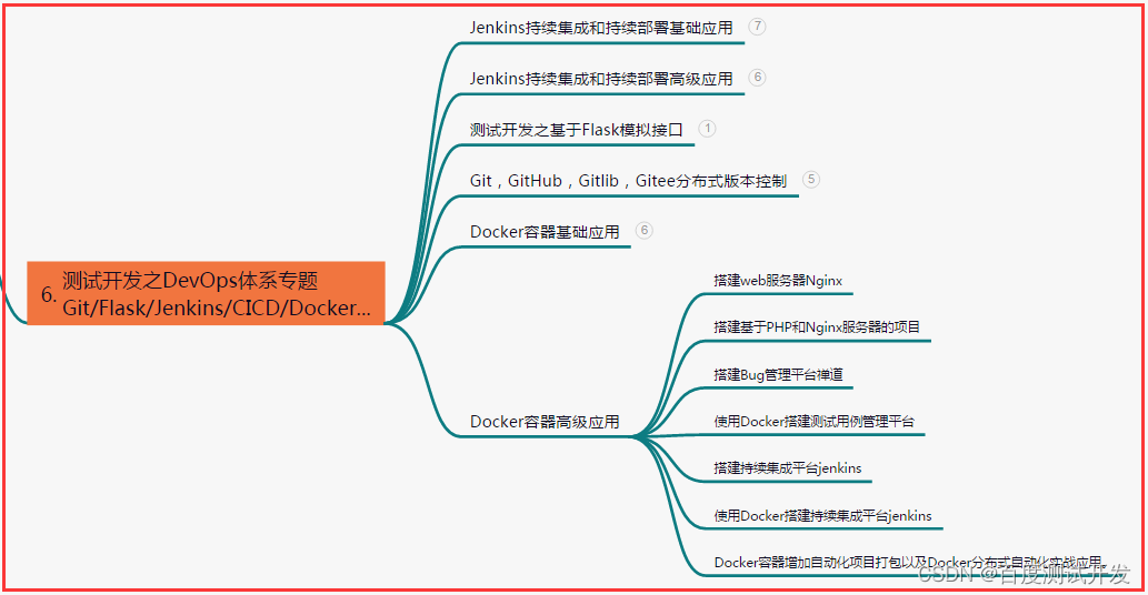
- 六、测试开发DevOps体系
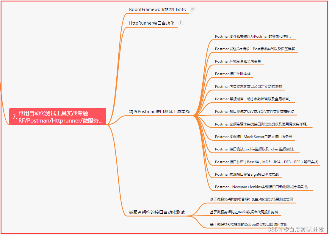
- 七、常用自动化测试工具
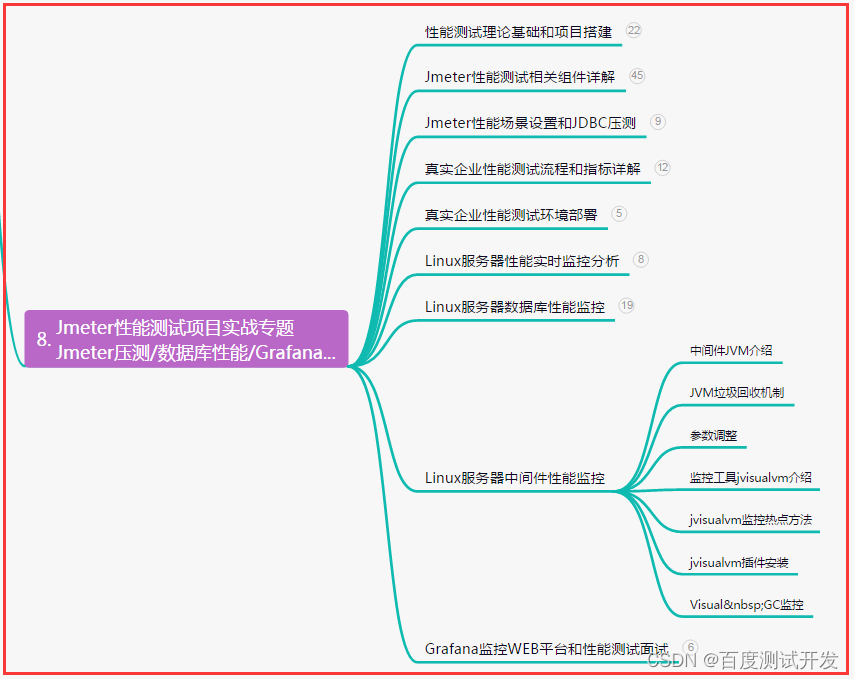
- 八、JMeter性能测试
- 九、总结(尾部小惊喜)
前言
测试流程(各有千秋)
1、测试人员参与需求评审、交互评审、视觉评审;理解需求,进行需求分析。
2、测试负责人编写测试计划,分配测试任务,评估测试周期。
3、测试人员整理交互or需求疑难点,确认异常场景or特殊情况下的交互细节,最好是能划出新功能的数据流图&流程图。
4、测试人员编写测试点,转化测试用例,评审测试点or测试用例。
5、开发送测(提测)前,开发自行走查,产品视觉验收,若有必要,测试可介入冒烟测试。
6、送测(提测)阶段,缺陷管理,发现bug,提交bug。
7、可以分A1,A2,A3…阶段,一般A1新功能测试用例&主流程回归,A2验证bug&交叉测试&拓展测试,A3验证bug&拓展测试。
8、预发(灰发)环境验证。
9、线上环境验证。
10、版本复盘。
自动化测试(分析与实施)
优点:
1、回归测试更方便,由于回归测试的额动作和用例是完全设计好,测试结果也是可以预料的,将回归测试自动运行,可以提高测试效率,缩短回归测试时间;
2、运行更多更繁琐的测试;
3、可以执行一些手工测试困难的测试,可以通过自动化测试模拟同时有大量用户的测试;
4、测试具有一致性和可重复性,每次测试的结果和执行的内容的一致性可以得到保障,达到测试的可重复的效果;
5、测试的复用性,实现在不同的测试过程中使用相同的用例;
6、测试的执行可靠性,按脚本执行,后续定位复现有明确的路径可循;
7、资源利用率高,人力成本低;
8、基本的、逻辑性不强的操作,性能测试、压力测试、回归测试,自动化测试很大优势。
缺点:
1、手工测试比自动测试发现的缺陷更多;
2、对测试的依赖性大;
3、只适合回归测试;
4、手工测试编写时间少于测试脚本编写时间;
5、手工测试可以靠人的想象力去测试, 而工具是死的;
6、自动化测试可能会制约软件开发,脚本维护会受到限制,从而制约软件的开发。
总结:自动化测试是对手工测试的一种补充,自动化测试不可能完全替代手工测试,因为很多数据的正确性、界面是否美观、业务逻辑的满足程度等都离不开测试人员的人工判断。
测试用例
1、基本的测试用例设计方法
基本的测试用例设计方法(边界值分析、等价类划分等)。
业务和场景的积累,了解测试需求以及易出现的bug的地方。
多维角度设计测试用例(用户、业务流程、异常场景、代码逻辑)。
2、需求分析
获取原始需求,结合实际场景确保需求描述的完整性。
需求产生的原因和价值(产品需求/研发需求;优化迭代、老应用增加新功能、新系统开发)。
不同类型的需求侧重不同的测试点(运营功能、JSF接口、定时任务等)。
3、测试用例设计
通过需求评审、业务和场景的积累、结合开发与产品的文档资料、以及通过多渠道学习测试用例设计方法,完成测试用例的设计。
测试用例模板:标题、配置条件(测试工具、中间件的使用情况)、测试数据、用例执行的先后顺序(先冻结再解冻,需对原单号进行解冻、用例的优先级)、预期结果(错误场景返回结果是否合理)等。
根据不同的需求测试类型(JSF接口测试、页面测试、新增数据表、JDOS迁移等类型)总结测试用例模板。
用例执行
利用各类测试手段(如deeptest平台、java+testNG框架、schedule等)执行测试用例,快速定位bug。
bug分类(前端bug/后端bug、测试平台的问题/需求bug、测试脏数据、日志缓存过多)。
bug复现(重复执行原测试操作、是否为数据库中的脏数据、前后端交互界面考虑网络问题等)。
测试效率提升
通过业务积累和测试工具的掌握,提升工作效率,如京东小店账务系统的改动(11个接口)四天左右测试完成,并提前上线。
总结各类测试用例模板。
明确与工作交接伙伴沟通的重点与方式。
沟通协调
掌握开发知识与业务知识的专业术语,提升沟通效率。
记录多个问题,一并沟通。
沟通方式方面,先保证测试步骤是正确的,将bug截图、日志错误、问题描述精准表述。
保证交流的焦点集中在急需解决的问题上。
开发人员的表述,保持高度警惕和怀疑精神,亲自验证及分析后再判断。
难以复现的bug,确定bug类型,找出原因,确保满足时限要求。
| 下面是我整理的2023年最全的软件测试工程师学习知识架构体系图 |
一、Python编程入门到精通
二、接口自动化项目实战
三、Web自动化项目实战
四、App自动化项目实战
五、一线大厂简历
六、测试开发DevOps体系
七、常用自动化测试工具
八、JMeter性能测试
九、总结(尾部小惊喜)
有志者,事竟成,破釜沉舟,百二秦关终属楚;苦心人,天不负,卧薪尝胆,三千越甲可吞吴。永不满足是我向上的动力。
希望是本无所谓有,无所谓无的。这正如地上的路,其实地上本没有路,走的人多了,也便成了路。有了梦想,就要不断的去追逐。这样,梦想才有可能实现。
生活的漫无目的一般都是因为缺乏目标感造成的。想要改变现状,要先告诉自己前进的最终目标和方向。