商业网站建站杭州网站建设宣盟网络
流媒体协议
元宇宙业务场景对流媒体传输的实时性和互动性提出了更高的要求,这就需要在传统的 RTMP、SRT、 HLS 等基础上增加实时互动的支持。实时互动,指在远程条件下沟通、协作,可随时随地接入、实时地传递虚实融合的多维信息,身临其境的交互体验。实时互动作为下一代互联网基础设施,实现了从“在线”到“在场” 的重要转变,将推动互联网向以“临场感”为主要特征的元宇宙方向的升级变革,当前几个主流的技术方向如下。

MPEG-DASH 是一项基于 HTTP 的动态自适应流传输技术,由 MPEG 在 2012 年推出。它不限制编码格式及内容,能够根据当前带宽容量、网络性能等情况自适应地实现不同码率之间的灵活切换,在为用户提供低卡顿体验的同时保证播放内容的质量。当前,MPEG-DASH 协议已成为全景视频的主要传输协议。
WebRTC 是一项实时通讯技术,早期由 Google 开源,实现了基于网页的实时通讯能力,并于 2021 年被万维网联盟(W3C)和互联网工程任务组(IETF)采纳为官方标准。WebRTC 可以实现超低延时、低卡顿的实时通讯效果,但是对虚拟现实内容面向元宇宙新的媒体类型媒体传输和交互支持不足。WebRTC-NV(Next Version)是下一代 WebRTC,是当前 WebRTC1.0 之后的标准,意在支持当前 WebRTC API 不可能或很难实现的新用例,比如 VR。主要是从通道扩展性、模块成熟和完善性、采集扩展性、独立的标准等 4 方面能力提升。
QUIC 是一项基于 UDP 的低时延通用传输协议,由 Google 推出,它从可靠传输、安全机制、时延等方面对 UDP 协议进行了优化,通过加密、流量控制、拥塞控制等技术,实现了更灵活、更安全、低时延的传输。目前,多个浏览器已支持 QUIC,比如 Google Chrome 浏览器、Microsoft Edge、Firefox 等。同时,该协议已广泛应用于移动端直播、短视频、高速图片文件下载等业务场景。
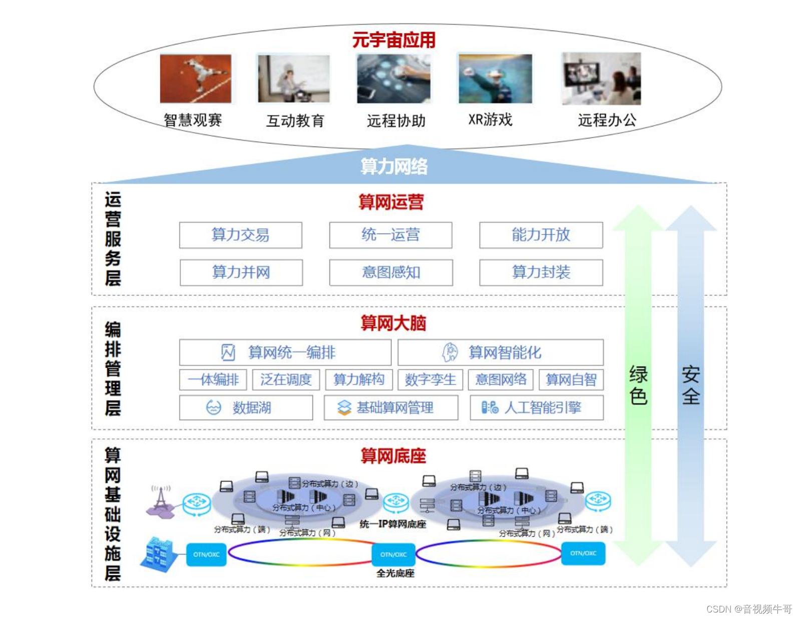
支撑元宇宙的算力网络架构图:
综上所述,面向未来元宇宙沉浸式体验的需求,3D 视觉媒体信息的低时延高效传输是亟需解决的问题。因此,如何基于 3D 视觉信息的特点对传输协议进行优化以实现低时延传输将是传输协议进一步发展的方向。
媒体传输
元宇宙场景中需要支持多种类型的视音频数据传输,以及对实时性、互动性有较高的要求。
3GPP SA4 正在进行 5G_RTP、iRTCW 、FS_ eiRTCW 等标准研究项目,将针对沉浸的实时业务(如 XR 业务)的沉浸媒体和相关元数据的实时传输,以及沉浸的实时通信。
同时,MPEG 已制定或正在制定支持元宇宙场景的全景视频、多视点视频、点云数据等沉浸媒体的传输标准,使用扩展的 DASH/MMT 协议传输 MPEG 的沉浸媒体封装文件。
IETF 和 W3C 组织于 2021 年将 WebRTC 采纳为官方标准,目前也正在研究下一代 WebRTC 标准。
WebRTC 工作组正在开发媒体捕获和媒体流以及屏幕捕获等规范,同时审阅支持 WebRTC 新用例的技术提案;探索边缘计算对 Web 平台的影响以及有关用例和需求,在 Web 浏览器中整合网络质量监测和预测。为支持元宇宙中不同场景的媒体传输,将对潜在的媒体传输协议的功能扩展并优化使用(如 RTP 协议、 WebRTC 协议)、传输的功能组件等进行标准研究,以及对元宇宙中潜在的、新兴的沉浸媒体数据格式提供灵活的传输/访问机制(如基于空间的媒体访问,基于视角的媒体传输)进行标准研究,以提高传输效率,减少终端开销,增加沉浸体验,满足不同的业务场景。