网站建制作公司万能搜索引擎网站
1写在前面
昨天又是不睡觉的一天,晚上还被家属讲了一通,理由是我去急诊了,没有在办公室待着,他老公疼没人去看。🫠
我的解释是只有我一个值班医生,不可能那么及时,而且也不是什么急症啊。😂
好的,说完家属就暴雷了,“这么大的医院就安排一个大夫值班吗!?”😡
我也是懒得跟她battle,这个世界不是谁生病就谁有理吧!~😂
今天继续接上一次monocle3的教程吧。🧐
2用到的包
library(tidyverse)
library(monocle3)
library(garnett)
3示例数据
还是上一次运行完的结果哦,不知道大家有没有保存。😂
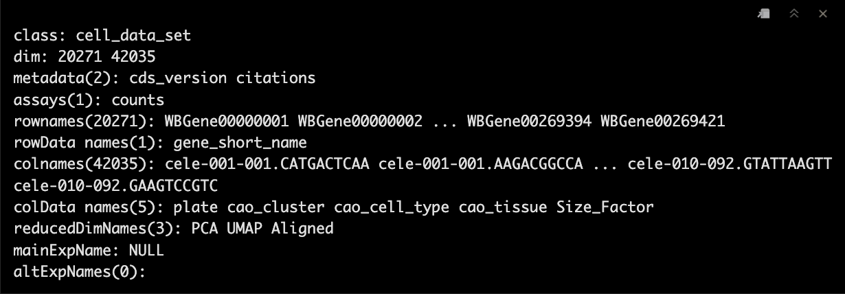
cds
4寻找marker genes
完成细胞聚类后,我们就可以使用top_markers()来选中marker genes。😘
marker_test_res <- top_markers(cds, group_cells_by="partition",
                               reference_cells=1000, cores=8)
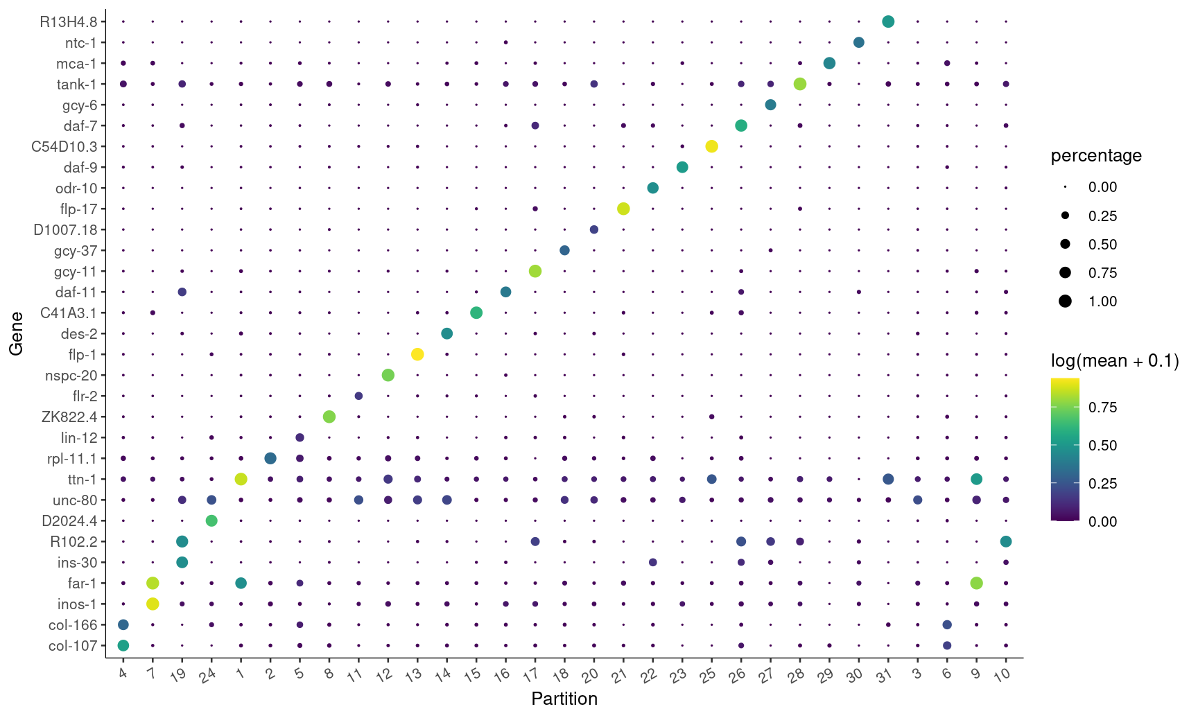
接着我们就可以根据cluster,partition或者colData(cds)来确定top n的基因表达量。🤩
top_specific_markers <- marker_test_res %>%
                            filter(fraction_expressing >= 0.10) %>%
                            group_by(cell_group) %>%
                            top_n(1, pseudo_R2)

top_specific_marker_ids <- unique(top_specific_markers %>% pull(gene_id))
可视化!~🤪
plot_genes_by_group(cds,
                    top_specific_marker_ids,
                    group_cells_by="partition",
                    ordering_type="maximal_on_diag",
                    max.size=3)
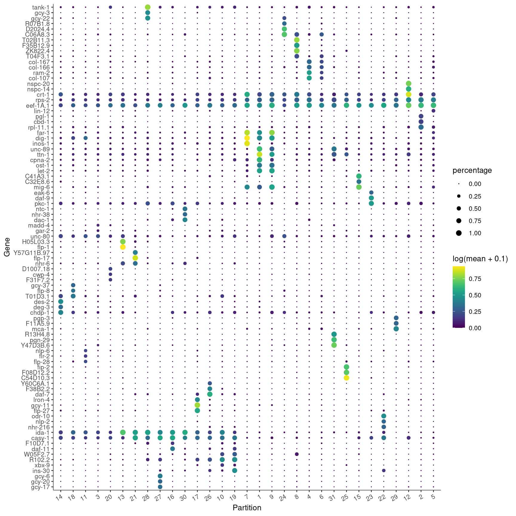
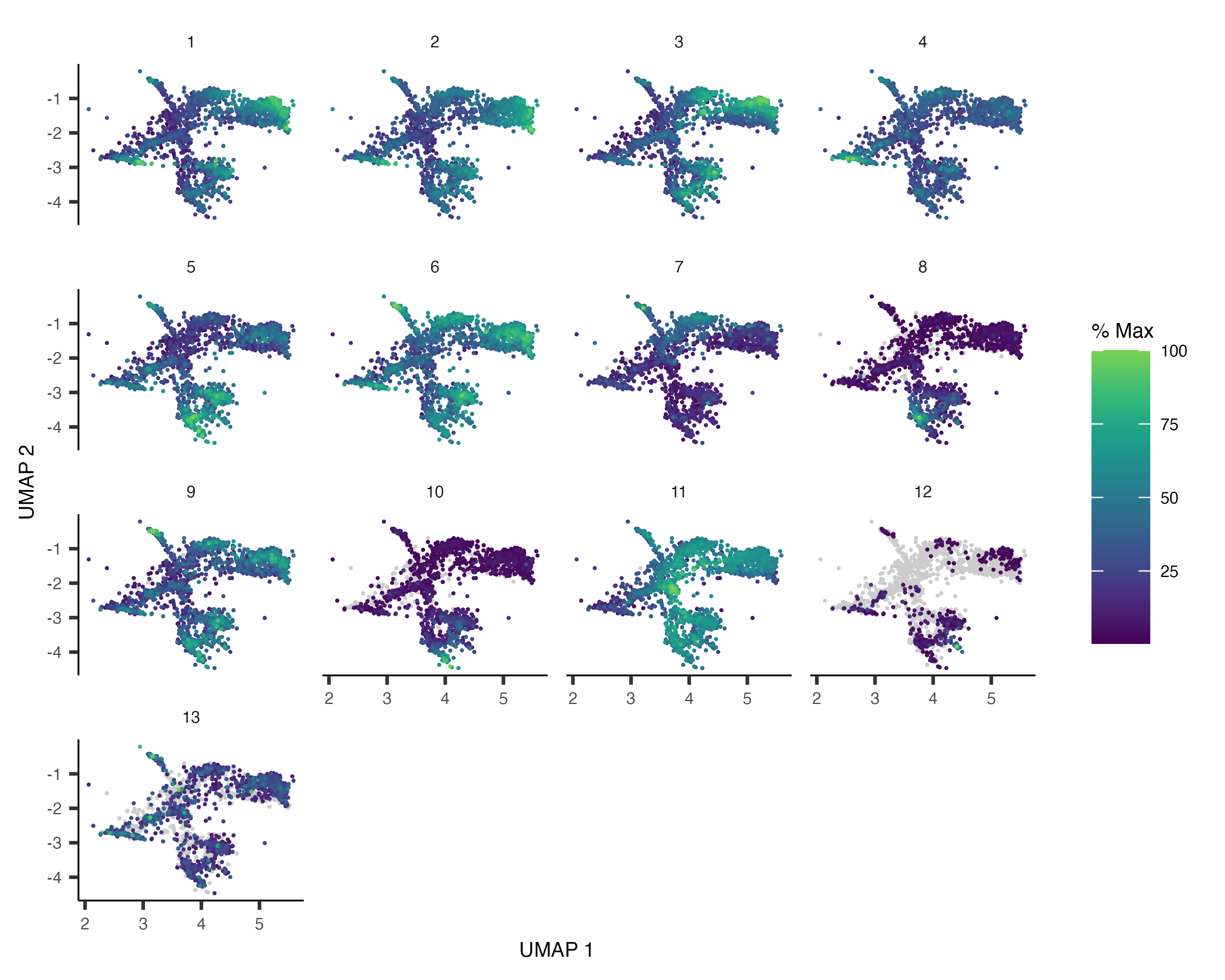
我们再试试看看top 3的基因。😘
top_specific_markers <- marker_test_res %>%
                            filter(fraction_expressing >= 0.10) %>%
                            group_by(cell_group) %>%
                            top_n(3, pseudo_R2)

top_specific_marker_ids <- unique(top_specific_markers %>% pull(gene_id))

plot_genes_by_group(cds,
                    top_specific_marker_ids,
                    group_cells_by="partition",
                    ordering_type="cluster_row_col",
                    max.size=3)
5注释细胞类型
确定每个cluster的类型对许多下游分析至关重要。😋
常用的方法是首先对细胞进行聚类,然后根据其基因表达谱为每个cluster注释一个细胞类型。😜
我们先创建一列新的colData。🤓
colData(cds)$assigned_cell_type <- as.character(partitions(cds))
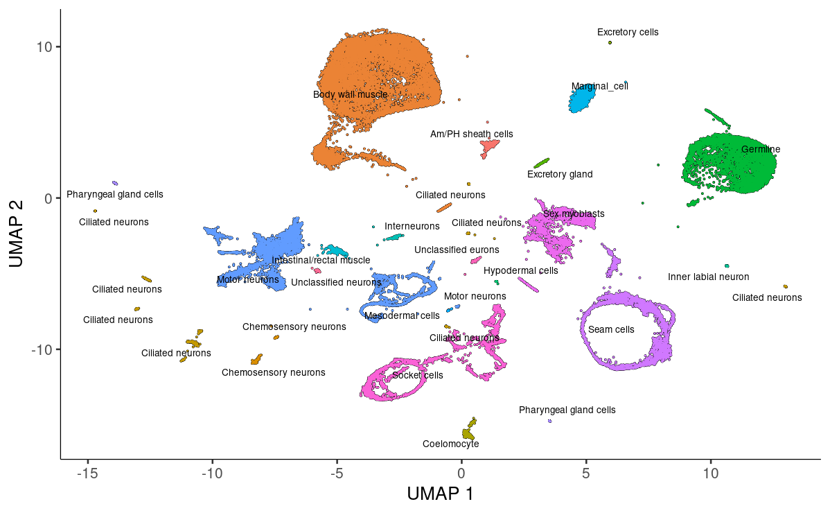
然后我们进行一下手动注释,其实手动注释是最准的。🧐
colData(cds)$assigned_cell_type <- dplyr::recode(colData(cds)$assigned_cell_type,
                                                 "1"="Body wall muscle",
                                                 "2"="Germline",
                                                 "3"="Motor neurons",
                                                 "4"="Seam cells",
                                                 "5"="Sex myoblasts",
                                                 "6"="Socket cells",
                                                 "7"="Marginal_cell",
                                                 "8"="Coelomocyte",
                                                 "9"="Am/PH sheath cells",
                                                 "10"="Ciliated neurons",
                                                 "11"="Intestinal/rectal muscle",
                                                 "12"="Excretory gland",
                                                 "13"="Chemosensory neurons",
                                                 "14"="Interneurons",
                                                 "15"="Unclassified eurons",
                                                 "16"="Ciliated neurons",
                                                 "17"="Pharyngeal gland cells",
                                                 "18"="Unclassified neurons",
                                                 "19"="Chemosensory neurons",
                                                 "20"="Ciliated neurons",
                                                 "21"="Ciliated neurons",
                                                 "22"="Inner labial neuron",
                                                 "23"="Ciliated neurons",
                                                 "24"="Ciliated neurons",
                                                 "25"="Ciliated neurons",
                                                 "26"="Hypodermal cells",
                                                 "27"="Mesodermal cells",
                                                 "28"="Motor neurons",
                                                 "29"="Pharyngeal gland cells",
                                                 "30"="Ciliated neurons",
                                                 "31"="Excretory cells",
                                                 "32"="Amphid neuron",
                                                 "33"="Pharyngeal muscle")
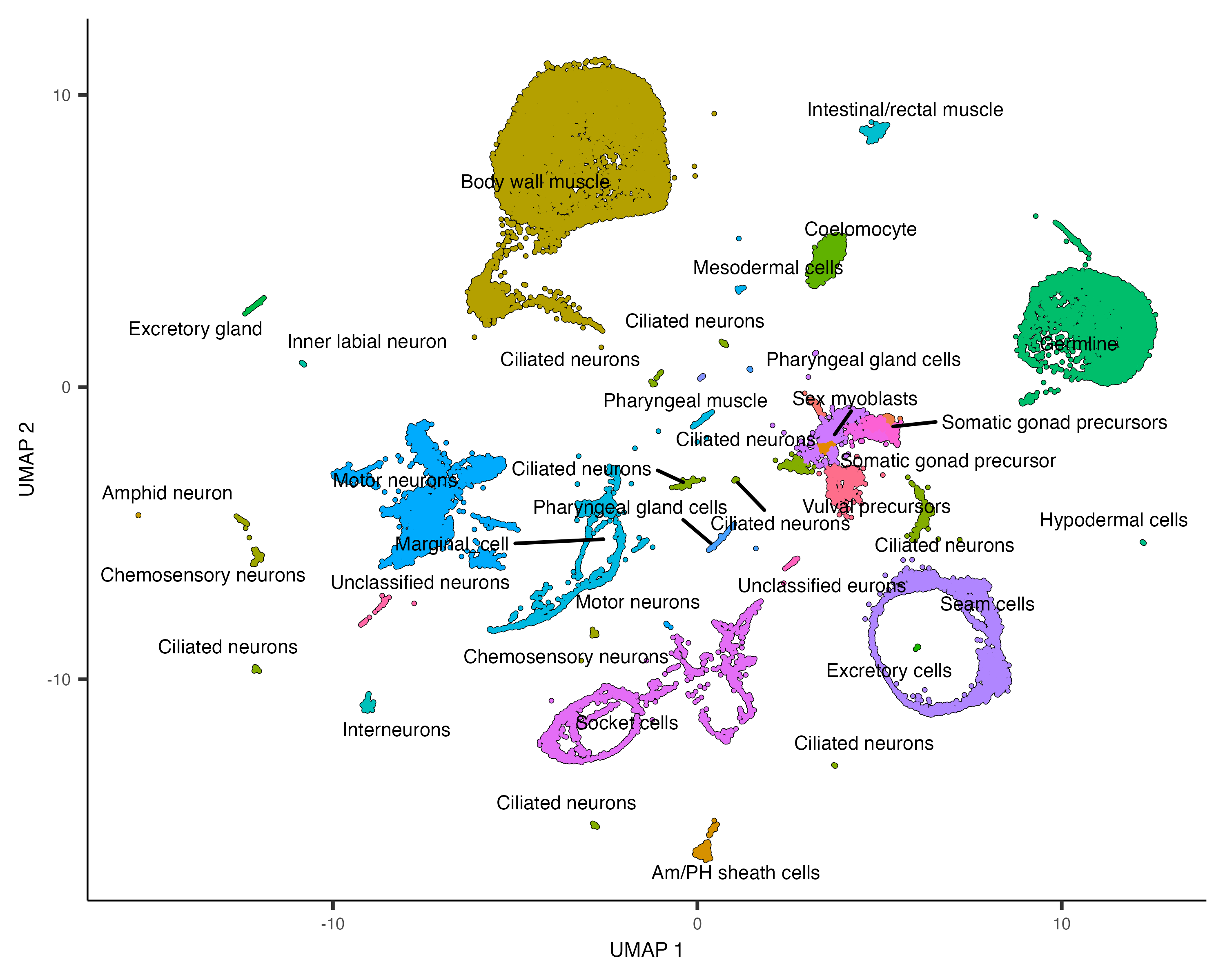
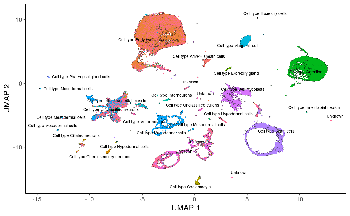
可视化咯!~🤣
plot_cells(cds, group_cells_by="partition", color_cells_by="assigned_cell_type")
我们可以利用choose_cells深入解析某个cluster中的亚群。😍
手动选择就行了,非常简单。🤣
cds_subset <- choose_cells(cds)
这个时候我们需要用到graph_test()取了解亚群之间的表达差异。🥸
pr_graph_test_res <- graph_test(cds_subset,
                                neighbor_graph= "knn",  #"knn", "principal_graph",
                                cores=8)

pr_deg_ids <- row.names(subset(pr_graph_test_res, morans_I > 0.01 & q_value < 0.05))
我们甚至可以把其中表达相似的基因归为一个module。😌
gene_module_df <- find_gene_modules(cds_subset[pr_deg_ids,], resolution=1e-3)
可视化module表达。🤩
plot_cells(cds_subset,
           genes=gene_module_df,
           show_trajectory_graph=F,
           label_cell_groups=F)
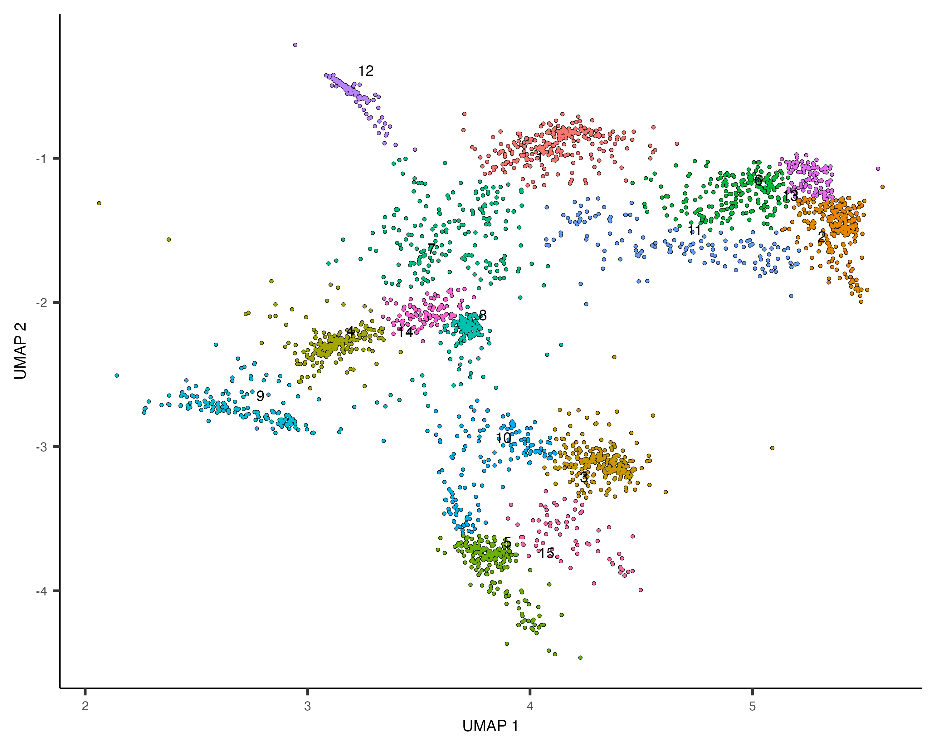
我们试试把分辨率再提高一些!~🧐
cds_subset <- cluster_cells(cds_subset, resolution=1e-2)

plot_cells(cds_subset, color_cells_by="cluster")
colData(cds_subset)$assigned_cell_type <- as.character(clusters(cds_subset)[colnames(cds_subset)])
colData(cds_subset)$assigned_cell_type <- dplyr::recode(colData(cds_subset)$assigned_cell_type,
                                                        "1"="Sex myoblasts",
                                                        "2"="Somatic gonad precursors",
                                                        "3"="Vulval precursors",
                                                        "4"="Sex myoblasts",
                                                        "5"="Vulval precursors",
                                                        "6"="Somatic gonad precursors",
                                                        "7"="Sex myoblasts",
                                                        "8"="Sex myoblasts",
                                                        "9"="Ciliated neurons",
                                                        "10"="Vulval precursors",
                                                        "11"="Somatic gonad precursor",
                                                        "12"="Distal tip cells",
                                                        "13"="Somatic gonad precursor",
                                                        "14"="Sex myoblasts",
                                                        "15"="Vulval precursors")

plot_cells(cds_subset, group_cells_by="cluster", color_cells_by="assigned_cell_type")
colData(cds)[colnames(cds_subset),]$assigned_cell_type <- colData(cds_subset)$assigned_cell_type
cds <- cds[,colData(cds)$assigned_cell_type != "Failed QC" | is.na(colData(cds)$assigned_cell_type )]
plot_cells(cds, group_cells_by="partition",
           color_cells_by="assigned_cell_type",
           labels_per_group=5)
6自动注释
这里我们用到的是Garnett。😀
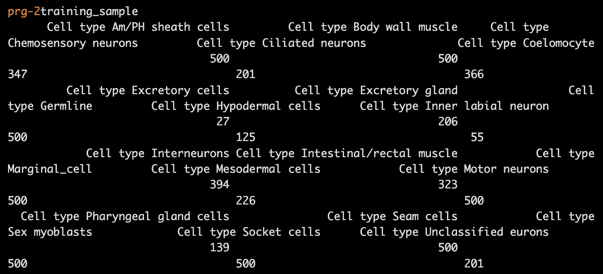
首先我们需要确定top_markers。🥸
assigned_type_marker_test_res <- top_markers(cds,
                                             group_cells_by="assigned_cell_type",
                                             reference_cells=1000,
                                             cores=8)
接着过滤一下marker genes。😚
过滤条件:👇
1️⃣ JS specificty score > 0.5;
2️⃣ logistic test 有意义;
3️⃣ 不是多个细胞类型的marker。
garnett_markers <- assigned_type_marker_test_res %>%
                        filter(marker_test_q_value < 0.01 & specificity >= 0.5) %>%
                        group_by(cell_group) %>%
                        top_n(5, marker_score)

garnett_markers <- garnett_markers %>%
                        group_by(gene_short_name) %>%
                        filter(n() == 1)
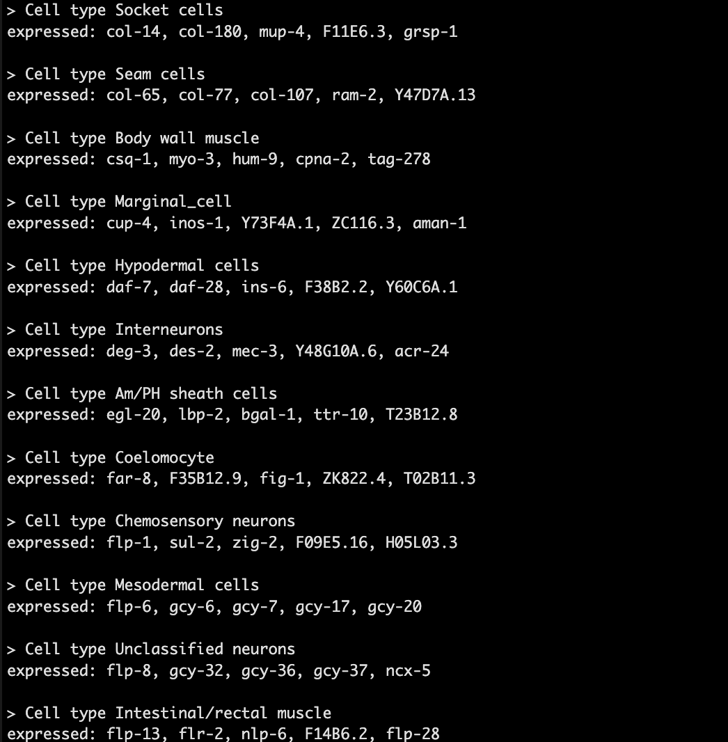
然后会生成一个marker文件。😏
这个文件你也可以进一步的加工一下,根据你的生物学背景等。😋
generate_garnett_marker_file(garnett_markers, file="./marker_file.txt")
现在可以注释咯,我们先训练一下classifier。🥸
colData(cds)$garnett_cluster <- clusters(cds)

worm_classifier <- train_cell_classifier(cds = cds,
                                         marker_file = "./marker_file.txt",
                                         db= org.Ce.eg.db::org.Ce.eg.db,
                                         cds_gene_id_type = "ENSEMBL",
                                         num_unknown = 50,
                                         marker_file_gene_id_type = "SYMBOL",
                                         cores=8)
现在可以使用前面训练好的worm_classifier了。😅
cds <- classify_cells(cds, worm_classifier,
                      db = org.Ce.eg.db::org.Ce.eg.db,
                      cluster_extend = TRUE,
                      cds_gene_id_type = "ENSEMBL")
可视化一下,果然还是挺适合我等懒🐶的!~🫠
plot_cells(cds,
           group_cells_by="partition",
           color_cells_by="cluster_ext_type")
线虫的现成模型,不需要自己训练了:👇
ceWhole <- readRDS(url("https://cole-trapnell-lab.github.io/garnett/classifiers/ceWhole_20191017.RDS"))
cds <- classify_cells(cds, ceWhole,
                      db = org.Ce.eg.db,
                      cluster_extend = TRUE,
                      cds_gene_id_type = "ENSEMBL")

点个在看吧各位~ ✐.ɴɪᴄᴇ ᴅᴀʏ 〰
📍 🤩 LASSO | 不来看看怎么美化你的LASSO结果吗!?
📍 🤣 chatPDF | 别再自己读文献了!让chatGPT来帮你读吧!~
📍 🤩 WGCNA | 值得你深入学习的生信分析方法!~
📍 🤩 ComplexHeatmap | 颜狗写的高颜值热图代码!
📍 🤥 ComplexHeatmap | 你的热图注释还挤在一起看不清吗!?
📍 🤨 Google | 谷歌翻译崩了我们怎么办!?(附完美解决方案)
📍 🤩 scRNA-seq | 吐血整理的单细胞入门教程
📍 🤣 NetworkD3 | 让我们一起画个动态的桑基图吧~
📍 🤩 RColorBrewer | 再多的配色也能轻松搞定!~
📍 🧐 rms | 批量完成你的线性回归
📍 🤩 CMplot | 完美复刻Nature上的曼哈顿图
📍 🤠 Network | 高颜值动态网络可视化工具
📍 🤗 boxjitter | 完美复刻Nature上的高颜值统计图
📍 🤫 linkET | 完美解决ggcor安装失败方案(附教程)
📍 ......


本文由 mdnice 多平台发布