模板网站有利于做seo吗阿里云虚拟主机wordpress建站教程

思路:需要一个二维数组dp来记录当前的公共子序列长度,如果当前的两个值等,则dp[i][j]=dp[i-1][j-1]+1,否则dp[i][j] = max(dp[i-1][j],dp[i][j-1])。也就是说,当前的dp值是由左、上、左上的值决定的。获得dp数组之后,倒序遍历这个二维数组,如果当前值和左边值相等,那就往左走,如果和上边值相等,就往上走,和左上值相等,就往左上走。并且保存当前的元素到ans中。最后将ans倒序输出。
class Solution:
def LCS(self , s1: str, s2: str) -> str:
n = len(s1)
m = len(s2)
if n <= 0 or m <= 0:
return '-1'
dp = [[0]*(m+1) for _ in range(n+1)]
ans = []
for i in range(n): #获取dp
for j in range(m):
if s1[i] == s2[j]:
dp[i+1][j+1] = dp[i][j]+1
else:
dp[i+1][j+1] = max(dp[i+1][j],dp[i][j+1])
a,b = n,m
while dp[a][b] != 0: #倒序遍历dp,取元素
if dp[a][b-1] == dp[a][b]: #该元素是从左边过来的
b -= 1
elif dp[a-1][b] == dp[a][b]: #该元素是从右边过来的
a -= 1
elif dp[a-1][b-1]+1 == dp[a][b]: #该元素是从左上过来的
a -= 1
b -= 1
ans.append(s1[a])
return ''.join(ans[::-1]) if len(ans) != 0 else '-1'
思路:子串一定是连续的,所以只需要记录dp[i+1][j+1] = dp[i][j]+1,其余都是0,每次更新值都要记录当前的最大长度和当前的结束位置。最后直接输出s1[index+1-res,index+1]即可。
class Solution:
def LCS(self, str1: str, str2: str) -> str:
n = len(str1)
m = len(str2)
if n <= 0 or m <= 0:
return ''
dp = [[0] * (m + 1) for _ in range(n + 1)]
res = 0
index = 0
for i in range(n):
for j in range(m):
if str1[i] == str2[j]:
dp[i + 1][j + 1] = dp[i][j] + 1
if res < dp[i+1][j+1]:
res = dp[i+1][j+1]
index = i
return str1[index+1-res:index+1]
但是这个方法会超时,可以使用值遍历一次的方法,寻找一个index,使得s1[index-maxlen,index+1]在s2中,更新maxlen和res继续寻找。
class Solution:
def LCS(self , str1: str, str2: str) -> str:
#让str1为较长的字符串
if len(str1) < len(str2):
str1, str2 = str2, str1
res = ''
max_len = 0
#遍历str1的长度
for i in range(len(str1)):
if str1[i - max_len : i + 1] in str2: #查找是否存在
res = str1[i - max_len : i + 1]
max_len += 1
return res

思路:由于机器人只能往右或者往下走,所以一个格子的路径等于它上边+左边的路径数。第一个格子的路径置为1,计算dp。
class Solution:
def uniquePaths(self , m: int, n: int) -> int:
if n <= 1 or m <= 1:
return 1
dp = [[0]*(n+1) for _ in range(m+1)]
dp[1][1] = 1
for i in range(1,m+1):
for j in range(1,n+1):
if i == 1 and j == 1:
continue
dp[i][j] = dp[i-1][j] + dp[i][j-1]
return dp[-1][-1]
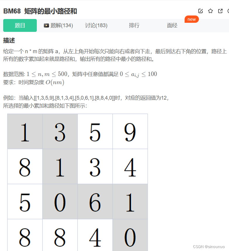
思路:从左上角走,只能向右或者向下走,对于第一列的格子,最小值一定是上面的权重加上当前权重,对于第一行的格子,最小值是左边的权重加上当前的权重。其他格子是左边或者上边的最小值加上当前权重。用dp保存每个格子的最小值,输出dp的最后一个值。
class Solution:
def minPathSum(self , matrix: List[List[int]]) -> int:
n = len(matrix)
m = len(matrix[0])
if n <= 0 or m <= 0:
return 0
dp = [[0]*(m) for _ in range(n)]
dp[0][0] = matrix[0][0]
for i in range(n):
for j in range(m):
if i == 0 and j == 0:
continue
elif i == 0 and j != 0: #第一行
dp[i][j] = dp[i][j-1] + matrix[i][j]
elif i != 0 and j == 0: #第一列
dp[i][j] = dp[i-1][j] + matrix[i][j]
elif i-1 >= 0 and j - 1 >= 0: #其他格子
dp[i][j] = min(dp[i][j-1]+matrix[i][j],dp[i-1][j]+matrix[i][j])
return dp[-1][-1]
思路:首先要判断字符串不能有前导0,不能为0。然后遍历传入的字符串(1,n),对当前字符串进行分类,如果是0,i-1是[1,2]说明该位置只能一种编码dp[i+1]=dp[i],如果是其他字符,就直接返回0。当前值是[1-6],如果i-1是[1,2],那该位置是两种编码dp[i+1]=dp[i]+dp[i-1],其他字符就是只有一种编码。当前值是[7-9],如果i-1是1,有两种编码,其他字符一种编码。
class Solution:
def solve(self , nums: str) -> int:
n = len(nums)
if n <= 0:
return 0
#判断前导0和值为0
if len(str(int(nums))) != len(nums) or int(nums) == 0: return 0
dp = [1]*(n+1)
for i in range(1,n):
if nums[i] == '0': #当前是0
if nums[i-1] in ['1','2']: dp[i+1] = dp[i] #合法情况一种编码
else: return 0 #其他返0
elif '1' <= nums[i] <= '6': #当前是1-6
if nums[i-1] in ['1','2']: dp[i+1] = dp[i-1] + dp[i] #两种编码
else: dp[i+1] = dp[i] #一种编码
elif '7' <= nums[i] <='9': #当前是7-9
if nums[i-1] == '1': dp[i+1] = dp[i] + dp[i-1] #两种编码
else: dp[i+1] = dp[i] #一种编码
return dp[-1]
思路:dp[i]为凑出i元需要的最少货币数,想要凑出aim元,最多需要aim个货币。dp的初始值为aim+1(该值不可能被取到)。遍历[1-aim]的钱数,再遍历arr中的面值,当前面值小于等于钱数才能使用该面值。dp[i]=min(dp[i],dp[i-j]+1)。最后输出dp[-1]如果该值小于等于aim,说明该值被是合法值。否则说明凑不出这个钱,返回-1.
class Solution:
def minMoney(self , arr: List[int], aim: int) -> int:
#特殊情况判断
if len(arr) <= 0 and aim > 0: return -1
if aim == 0: return 0
if aim < min(arr): return -1
#设置dp,dp[i]表示达i元需要dp[i]的货币数
dp = [aim+1 for _ in range(aim+1)]
dp[0] = 0
#遍历钱数
for i in range(1,aim+1):
#遍历面值
for j in arr:
if j <= i: #当面值小于等于i元才能用该面值
dp[i] = min(dp[i],dp[i-j]+1)
return dp[-1] if dp[-1] <= aim else -1 #对最后的值判断再输出

思路:遍历两次数组,对于 i 的前面的数 j ,如果num[j]<num[i],就更新dp的值。dp[i] = max(dp[i],dp[j]+1),并且更新此时的ans,ans = max(ans,dp[i])
class Solution:
def LIS(self , arr: List[int]) -> int:
if len(arr) <= 1:
return len(arr)
dp = [1]*len(arr)
ans = 0
for i in range(len(arr)):
for j in range(i):
if arr[j] < arr[i]:
dp[i] = max(dp[i],dp[j]+1)
ans = max(ans,dp[i])
return ans
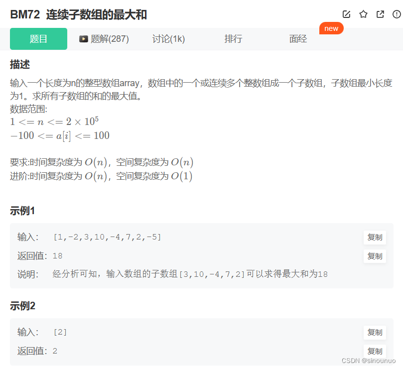
思路:当前的最大和,要么是前面的和+当前值,要么是当前值。dp[i] = max(array[i],dp[i-1]+array[i]),最后输出max(dp)。
class Solution:
def FindGreatestSumOfSubArray(self , array: List[int]) -> int:
if len(array) <= 1:
return array[0]
dp = []
dp.append(array[0])
for i in range(1,len(array)):
dp.append(max(array[i],dp[i-1]+array[i]))
return max(dp)

思路:回文子串有两种可能:bab,或者baab,也就是从一个字符串往两边延伸,可能获得一个回文串,或者用两个字符串往两边延伸也可能获得回文串。遍历每个字符,计算两种可能的回文串长度,并且和当前答案比较,如果大,就更新答案。
class Solution:
def length(self,A,left,right):
while left >= 0 and right < len(A) and A[left] == A[right]: #符合回文串
left -= 1
right += 1
return right -1 - left #(right-1)-(left+1)+1,当前回文串长度
def getLongestPalindrome(self , A: str) -> int:
if len(A) <= 1:
return len(A)
ans = 0
for i in range(len(A)):
ans = max(ans,self.length(A,i,i),self.length(A,i,i+1))
return ans
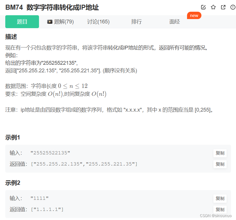
思路:循环分割,每次判断前导0和255大小。
class Solution:
def restoreIpAddresses(self , s: str) -> List[str]:
if len(s) == 0:
return []
ans = []
for i in range(1,len(s)-2):
for j in range(i+1,len(s)-1):
for k in range(j+1,len(s)):
a,b,c,d = s[:i],s[i:j],s[j:k],s[k:]
if len(str(int(a))) != len(a) or len(str(int(b))) != len(b) or len(str(int(c))) != len(c) or len(str(int(d))) != len(d): #前导0
continue
elif int(a) > 255 or int(b) > 255 or int(c) > 255 or int(d) > 255 : #判断和255大小
continue
else:
ans.append('.'.join([a,b,c,d]))
return ans

思路:dp[i]=max(dp[i-1],dp[i-2]+nums[i])
class Solution:
def rob(self , nums: List[int]) -> int:
n = len(nums)
dp = [0]*n
for i in range(n):
if i == 0:
dp[i] = nums[i]
elif i == 1:
dp[i] = max(nums[i-1],nums[i])
elif i >= 2:
dp[i] = max(dp[i-1],dp[i-2]+nums[i])
return dp[-1]
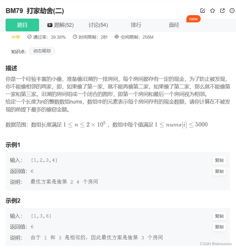
思路:和前一个题的思路,不同之处在于环,所以有两种情况:
第一家偷了,就不能偷最后一家,最大值是倒数第二家的最大值;
第一家不偷,可以投最后一家,最大值是倒数第一家的最大值。
class Solution:
def rob(self , nums: List[int]) -> int:
n = len(nums)
#环形的主要区别是,偷第一家就不偷最后一家,偷最后一家就不偷第一家
dp1 = [0]*n
dp2 = [0]*n
#一定偷第一家
dp1[0] = nums[0]
for i in range(1,n):
if i == 1:
dp1[i] = dp1[i-1]
else:
dp1[i] = max(dp1[i-2]+nums[i],dp1[i-1])
#一定偷最后一家
dp2[0] = 0
for i in range(1,n):
if i == 1:
dp2[i] = nums[i]
else:
dp2[i] = max(dp2[i-2]+nums[i],dp2[i-1])
return max(dp1[-2],dp2[-1]) #dp1最后一家不能偷,所以只能拿倒数第二家的最大值

思路:只能买卖一次的情况下,如果当前是i,选择[0-i]的最小值,[i:len-1]的最大值,ans表示两者之差,如果差值变大就更新ans。
class Solution:
def maxProfit(self , prices: List[int]) -> int:
ans = 0
for i in range(len(prices)):
a = min(prices[:i+1]) #[0,i]
b = max(prices[i:]) #[i,len-1]
ans = max(ans,b-a)
return ans
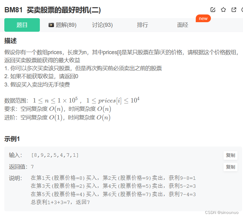
思路:可以有多次买卖股票的情况下,当前是第i天,在当前能够得到的最大获利分为两种情况,第一种是今天持有股票:dp[i][1] = max(dp[i-1][1],dp[i-1][0]-prices[i])要么前一天也持有,今天就不变,要么前一天不持有,今天就购买。第二种是今天不持有股票,要么前一天也不持有,今天不变,要么前一天持有,今天卖出。dp[i][0] = max(dp[i-1][0],dp[i-1][1]+prices[i]),返回最后一天不持有的数值。
class Solution:
def maxProfit(self , prices: List[int]) -> int:
n = len(prices)
if n <= 1:
return 0
dp = [[0,0] for _ in range(n)]
for i in range(len(prices)):
if i == 0:
dp[i][0] = 0
dp[i][1] = -prices[i]
else:
dp[i][0] = max(dp[i-1][0],dp[i-1][1]+prices[i])
dp[i][1] = max(dp[i-1][1],dp[i-1][0]-prices[i])
return dp[-1][0]
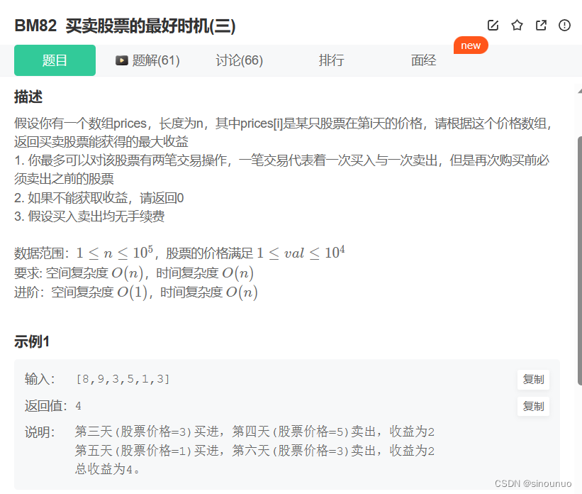
思路:因为只能买两次,所以本次状态转移就有五个选择
- dp[i][0]表示到第i天为止没有买过股票的最大收益
- dp[i][1]表示到第i天为止买过一次股票还没有卖出的最大收益
- dp[i][2]表示到第i天为止买过一次也卖出过一次股票的最大收益
- dp[i][3]表示到第i天为止买过两次只卖出过一次股票的最大收益
- dp[i][4]表示到第i天为止买过两次同时也买出过两次股票的最大收益
class Solution:
def maxProfit(self , prices: List[int]) -> int:
n = len(prices)
if n <= 3:
return 0
dp = [[-10000]*5 for i in range(n)]
dp[0][0] = 0
dp[0][1] = -prices[0]
for i in range(1,n):
dp[i][0] = dp[i-1][0]
dp[i][1] = max(dp[i-1][1],dp[i-1][0]-prices[i])
dp[i][2] = max(dp[i-1][2],dp[i-1][1]+prices[i])
dp[i][3] = max(dp[i-1][3],dp[i-1][2]-prices[i])
dp[i][4] = max(dp[i-1][4],dp[i-1][3]+prices[i])
return dp[-1][4]
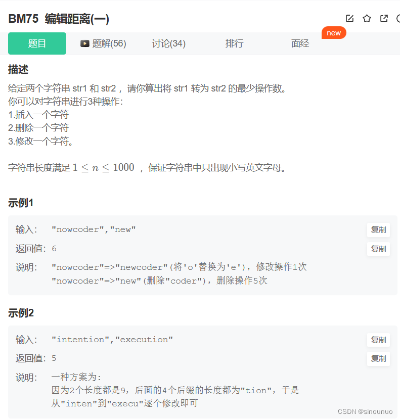
思路:两个字符串或者两个数组来确定相同子串或者改成相同,都按照二维dp思考,如果当前两个子串的对应位置不等,那该处的最小值是左、上、左上的最小值+1,如果等,就是左上对角线的值。
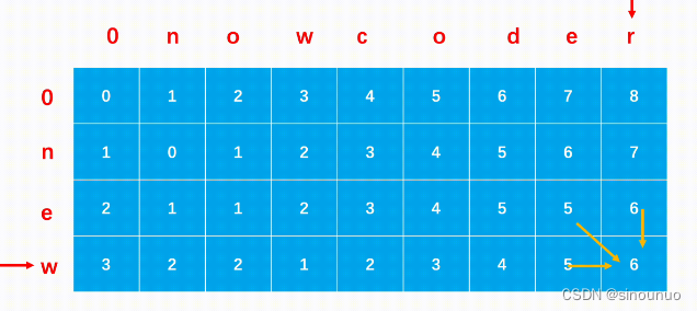
class Solution:
def editDistance(self , str1: str, str2: str) -> int:
n = len(str1)
m = len(str2)
dp = [[0]*(m+1) for _ in range(n+1)]
for i in range(n+1):
for j in range(m+1):
if i == 0:
dp[i][j] = j
elif j == 0:
dp[i][j] = i
else:
if str1[i-1] != str2[j-1]:
dp[i][j] = min(dp[i-1][j-1],dp[i-1][j],dp[i][j-1])+1
else:
dp[i][j] = dp[i-1][j-1]
return dp[-1][-1]
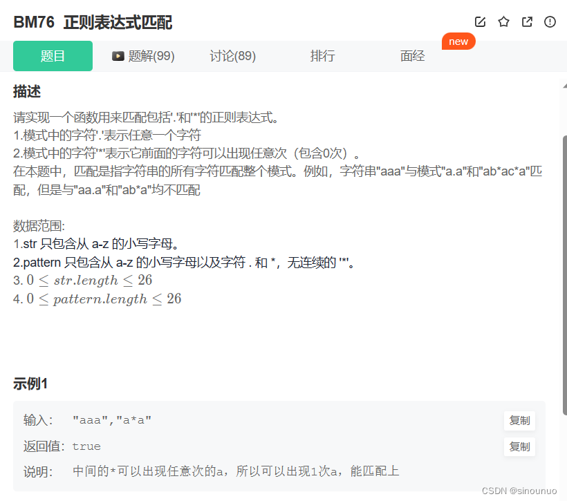
思路:首先进行长度异常判断,如果没有模式长度,那字符串长度也应该为空。然后开始匹配字符串和模式的第一位first_match。然后递归匹配之后的情况,如果第二位出现了*,那第一位不匹配也没有关系,匹配(s,pattern[2:]),如果第一位匹配,就匹配之后的(s[1:],pattern)。
如果第二位没有*,就递归first_match和(s[1:],pattern[1:])
class Solution:
def match(self , s: str, pattern: str) -> bool:
if not pattern : return not s
first_match = s and pattern[0] in [s[0],'.']
if len(pattern) >= 2 and pattern[1] == '*':
return self.match(s,pattern[2:]) or first_match and self.match(s[1:],pattern)
else:
return first_match and self.match(s[1:],pattern[1:])

思路:使用栈,让栈顶是当前没有匹配的括号的下标,保证栈不空,将-1先入栈。首先遇到'('就让左括号的下标入栈,如果遇到')',如果当前栈的长度大于1(已经有左括了),就弹出栈顶做匹配,res更新为max(res,i - stack[-1]);如果当前长度不大于1(没有左括号),就更新栈顶为当前没有匹配的右括号的下标(stack[-1] = i)
class Solution:
def longestValidParentheses(self , s: str) -> int:
stack = [-1]
res = 0
for i,ch in enumerate(s):
if ch == '(':
stack.append(i) #左括号下标入栈
else:
if len(stack) > 1:
stack.pop()
res = max(res,i - stack[-1])
else:
stack[-1] = i
return res