计算机网站设计论文企业策划工作内容
C++中拷贝构造和赋值重载的注意事项以及编译器的优化处理
- 前言
- 1. 拷贝构造和赋值重载的易混淆点和注意事项
- 1.1 易混淆点
- 1.2 注意事项
- 2.编译器对拷贝构造和赋值重载的优化处理
前言
本文可以帮助你对下面:
(1)何时调用拷贝构造何时调用赋值重载
(2)在拷贝构造函数和赋值重载函数的参数加const的意义
(3)自定义类型的隐式类型转换
(4)编译器对自定义类型隐式类型转换的优化
(5)自定义类型引用常量的意义
方面有更加深刻的理解
1. 拷贝构造和赋值重载的易混淆点和注意事项
1.1 易混淆点
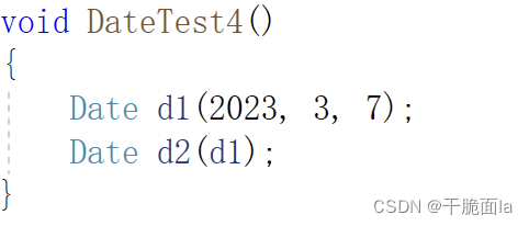
上图代码中的Date d2(d1);这句话大家可以很快就判断出是拷贝构造。
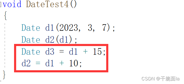
上图代码中的Date d3 = d1 + 15;是拷贝构造,Date d2 = d1 + 10;是赋值重载
原因如下:
(1)由于d3是为初始化的Date对象并用d1+15来初始化,即使使用等号来初始化,编译器还是会识别它为拷贝构造,相当于把Date d3 = d1 + 15;转化为Date d3(d1);因此是拷贝构造。
(2)然而d2是已经存在的对象,并用d1+10来赋值因此是赋值重载。
1.2 注意事项
拷贝构造和赋值重载函数的参数,最好加const,否则以上面的例子为例,可能会出错:
以代码Date d3 = d1 + 15;为例:

如上图首先先调用运算符重载operator+,由于ret是operator+里的局部变量,出了作用域就会自动删除,因此会先将ret拷贝到临时对象后才返回值(调用了拷贝构造),而临时对象为右值,具有常性(相当于用const修饰),这个临时对象又作为拷贝构造函数的参数,由于参数的类型是const Date,而拷贝构造函数需要接收Date&类型的参数,存在引用的权限放大的问题,因此编译器会报错!
同理,Date d2 = d1 + 10;也会报错。
所以我们习惯在拷贝构造和赋值重载函数的参数中为其添加const进行修饰,有两个好处:
(1)防止误写入
(2)避免权限放大问题

2.编译器对拷贝构造和赋值重载的优化处理

观察上面的两句话,第一句Date d1(2022);是大家熟知的构造函数
让人疑惑的是第二句Date d2(2022);中的Date类型的d2为什么能用int类型的2022来赋值呢?
其实这里是隐式类型的转化,在类的构造函数没有被explicit修饰的时候,编译器允许这种转化。
也就是把2022这个整形变量隐式转化为Date类型的变量。隐式类型转化的步骤如下:
(1)传一个参数调用构造函数来初始化一个const Date类型的临时对象
(2)调用Date的拷贝构造函数,将临时对象作为拷贝构造函数的参数,从而初始化d2.

也就是说,Date d2 = 2022;这个语句会先调用一次构造函数,再调用一次拷贝构造函数,但是大胆点的编译器(如VS2019)会对其步骤进行优化,对其进行合二为一。
也就是直接将2022作为d2的构造函数的参数对d2进行初始化。

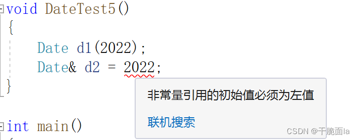
值得一提的是,在对int类型的常量2022进行引用操作的时候,编译器就会老老实实按照创建临时对象并调用其构造函数进行初始化,类型为const Date。再对其进行引用。
因此Date& d2 = 2022;的写法是错误的,存在权限放大
正确的写法是const Date& = 2022;
实际意义可以体现在String类:
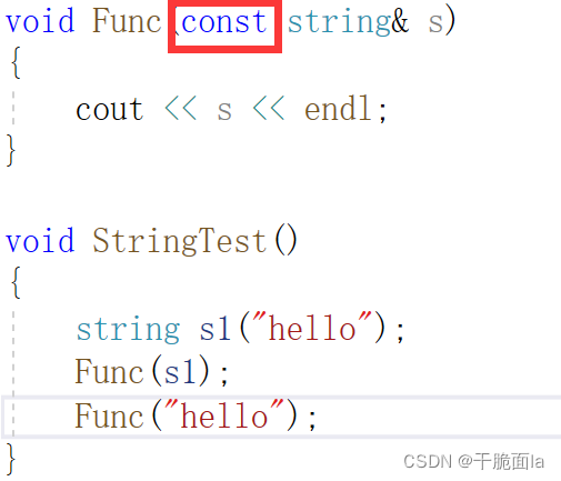
下图中的Func("hello");这句话就是用"hello"初始化了一个const String类的对象,因此用string来引用的时候会报错,要想用"hello"来调用Func函数的话,就必须加上const。
加上const前,编译器报错:

加上const后,可以正常调用: